Feedback 2
using DifferentialEquations
using OrdinaryDiffEq
using LinearAlgebra
using Random
using Plots
using LaTeXStrings
using Colors

include("common.jl")

default(fontfamily = "Computer Modern", framestyle = :box)
β = 0.8
γ = 0.2
S0 = 0.92
I0 = 0.04
Qbudget = 16.0
tf = 100.0
nothingThe herd-immunity threshold is
\[S_h=\frac{\gamma}{\beta}.\]
Sh = γ / β0.25Target levels
As in Feedback 1, the reference trajectory uses the target infection level computed from the estimated initial conditions $(\hat\theta_1,\hat\theta_2)$.
Define
\[I_h = \hat\theta_2+\hat\theta_1-S_h -S_h\log\left(\frac{\hat\theta_1}{S_h}\right).\]
The corresponding critical intervention budget is
\[Q_{\mathrm{crit}} = \frac{I_h-\hat\theta_2} {\beta S_h\hat\theta_2}.\]
The reference target value $I^\star$ is therefore defined by
\[I^\star= \begin{cases} \dfrac{I_h}{1+\beta S_hQ}, & Q<Q_{\mathrm{crit}},\\[2mm] \hat\theta_2, & Q\geq Q_{\mathrm{crit}}. \end{cases}\]
For Feedback 2, the feedback laws themselves use the constant lower bound
\[I_l= \frac{1-S_h+S_h\log S_h} {1+\beta S_h Q}.\]
function ISTAR(θ̂1::Real, θ̂2::Real)
    Ih = θ̂2 + θ̂1 - Sh - Sh * log(θ̂1 / Sh)

    Qcrit =
        (Ih - θ̂2) /
        (β * Sh * max(θ̂2, 1e-12))

    return Qbudget < Qcrit ?
           Ih / (1.0 + β * Sh * Qbudget) :
           θ̂2
end

Ibar = ISTAR(S0, I0)

Il =
    (1.0 - Sh + Sh * log(Sh)) /
    (1.0 + β * Sh * Qbudget)

nothing
Feedback laws
Two feedback laws are considered.
The first one is the NSN feedback control with the constant threshold $I_l$:
\[u_{2}(\hat I,\hat S):= \begin{cases} 1-\dfrac{S_h}{\hat S}, & \text{if } \hat I \geq I_l \text{ and } \hat S>S_h,\\[6pt] 0, & \text{otherwise}. \end{cases}\]
The second feedback is a modified version with an additional multiplicative term:
\[\widetilde u_{2}(\hat I,\hat S):= \begin{cases} 1-\dfrac{S_h}{\hat S}\dfrac{I_l}{\hat I}, & \begin{aligned} \text{if } \hat I \geq I_l \\ \text{and } \hat S > S_h, \end{aligned} \\[8pt] 0, & \text{otherwise}. \end{cases}\]
The additional term $I_l/\hat I$ in $\widetilde u_2$ amplifies the control value when $\hat I$ exceeds the threshold, forcing the infected trajectory to remain closer to the level $I_l$ while consuming more budget.
safe_ = 1e-10

@inline incidence(S, I, u) =
    β * S * I * (1.0 - u)

CONTROL_LAW = :u2:u2Possible values for CONTROL_LAW:
:u2:u2_tilde
u2_exact(Ŝ, Î) =
    (Ŝ ≤ Sh || Î < Il) ?
    0.0 :
    1.0 - Sh / Ŝ

u2_tilde_exact(Ŝ, Î) =
    (Ŝ ≤ Sh || Î < Il) ?
    0.0 :
    1.0 - (Sh / Ŝ) * (Il / Î)

ft_control(Ŝ, Î) =
    CONTROL_LAW === :u2 ?
    u2_exact(Ŝ, Î) :
    u2_tilde_exact(Ŝ, Î)

nothing
Smooth control used for the EKF
For the Extended Kalman Filter simulation, the discontinuous switching conditions are regularized.
We introduce
\[\sigma_\varepsilon(z) = \frac12 \left( 1+\tanh\left(\frac{z}{\varepsilon}\right) \right).\]
ϵ_I = 1e-2
ϵ_S = 1e-6

@inline function sigmoid_stable(z, ϵ)

    r = z / ϵ

    if r <= -40.0
        return 0.0
    elseif r >= 40.0
        return 1.0
    else
        return 0.5 * (1.0 + tanh(r))
    end
end
nothing
For $u_2$,
function nsn_u2(Ŝ, Î)

    Ssafe = max(Ŝ, safe_)

    σI = sigmoid_stable(
        Î - Il,
        ϵ_I
    )

    σS = sigmoid_stable(
        Ssafe - Sh,
        ϵ_S
    )

    return clamp(
        (1.0 - Sh / Ssafe) *
        σI *
        σS,
        0.0,
        1.0
    )
end
nothing
For $\widetilde u_2$,
function nsn_u2_tilde(Ŝ, Î)

    Ssafe = max(Ŝ, safe_)
    Isafe = max(Î, safe_)

    σI = sigmoid_stable(
        Î - Il,
        ϵ_I
    )

    σS = sigmoid_stable(
        Ssafe - Sh,
        ϵ_S
    )

    return clamp(
        (1.0 - Sh / Ssafe) *
        (Il / Isafe) *
        σI *
        σS,
        0.0,
        1.0
    )
end

nsn_control(Ŝ, Î) =
    CONTROL_LAW === :u2 ?
    nsn_u2(Ŝ, Î) :
    nsn_u2_tilde(Ŝ, Î)

nothing
Reference trajectory
The reference solution is divided into three phases.
Phase 1 — Uncontrolled epidemic
Initially,
\[u(t)=0.\]
The system therefore evolves according to
\[\begin{aligned} \dot S &= -\beta SI,\\ \dot I &= \beta SI-\gamma I. \end{aligned}\]
until the infection reaches the prescribed level $I^\star$.
tgrid = 0.0:0.05:tf

cb1 =
    ContinuousCallback(
        (v, t, integrator) ->
            v[2] - Ibar,
        terminate!
    )

sol1 = solve(
    ODEProblem(
        (dv, v, p, t) -> begin

            y = β * v[1] * v[2]

            dv[1] = -y
            dv[2] =  y - γ * v[2]
            dv[3] =  0.0

        end,

        [S0, I0, Qbudget],
        (0.0, tf)
    ),

    saveat = tgrid,
    callback = cb1,
    reltol = 1e-8,
    abstol = 1e-8
)
nothing
Phase 2 — Intervention arc
Once $I=I^\star$, the feedback
\[u(t)=1-\frac{S_h}{S(t)}\]
is applied.
The budget variable satisfies
\[\dot C(t)=-u(t).\]
The intervention ends either when the budget is exhausted or when $S=S_h$.
cb2_C =
    ContinuousCallback(
        (v, t, integrator) -> v[3],
        terminate!
    )

cb2_S =
    ContinuousCallback(
        (v, t, integrator) ->
            v[1] - Sh,
        nothing,
        terminate!
    )

cb2 = CallbackSet(cb2_C, cb2_S)

sol2 = solve(
    ODEProblem(
        (dv, v, p, t) -> begin

            S, I, C =
                v[1], v[2], v[3]

            u = 1.0 - Sh / S

            y = β * S * I

            dv[1] = -y * (1 - u)
            dv[2] =  y * (1 - u) - γ * I
            dv[3] = -u

        end,

        sol1.u[end],
        (sol1.t[end], tf)
    ),

    saveat = tgrid,
    callback = cb2,
    reltol = 1e-8,
    abstol = 1e-8
)
nothing
Phase 3 — Final uncontrolled trajectory
After the controlled phase,
\[u(t)=0\]
again.
sol3 = solve(
    ODEProblem(
        (dv, v, p, t) -> begin

            y = β * v[1] * v[2]

            dv[1] = -y
            dv[2] =  y - γ * v[2]
            dv[3] =  0.0

        end,

        sol2.u[end],
        (sol2.t[end], tf)
    ),

    saveat = tgrid,
    reltol = 1e-8,
    abstol = 1e-8
)
nothing
The three phases are concatenated as follows:
t_ref = [
    sol1.t;
    sol2.t[2:end];
    sol3.t[2:end]
]

S_ref = [
    sol1[1, :];
    sol2[1, 2:end];
    sol3[1, 2:end]
]

I_ref = [
    sol1[2, :];
    sol2[2, 2:end];
    sol3[2, 2:end]
]

C_ref = [
    sol1[3, :];
    sol2[3, 2:end];
    sol3[3, 2:end]
]

n1 = length(sol1.t)
n2 = length(sol2.t) - 1
n3 = length(sol3.t) - 1

u_ref = [
    zeros(n1);
    1.0 .- Sh ./ S_ref[n1+1:n1+n2];
    zeros(n3)
]
nothing
Extended Kalman Filter
We next compare the finite-time observer with a continuous-time Extended Kalman Filter.
Let
\[x= \begin{pmatrix} S\\ I \end{pmatrix}.\]
The measured quantity is the epidemic incidence
\[h(x,u) = \beta SI(1-u).\]
The EKF is written as
\[\dot{\hat x} = f(\hat x,u) + PH^\top R^{-1} \left( y-h(\hat x,u) \right),\]
with covariance equation
\[\dot P = AP+PA^\top - PH^\top R^{-1}HP + Q.\]
EKF parameters
R =
    1e-4

Qproc =
    Matrix(
        Diagonal(
            [1e-2, 1e-2]
        )
    )

P0 =
    Matrix(
        Diagonal(
            [1e-2, 1e-2]
        )
    )

Ŝ0, Î0 =
    1.0, 0.0

meas_noise_amp =
    0.1
nothing
Measurement noise
A deterministic multi-frequency signal is used to generate the measurement perturbation.
const NOISE_W =
    (
        0.17,
        0.41,
        0.93,
        2.13,
        3.71,
        7.29,
        11.93,
        19.07
    )

const NOISE_P =
    (
        0.00,
        1.13,
        2.47,
        0.62,
        4.01,
        5.28,
        1.97,
        3.55
    )

@inline function meas_noise(t)

    s = 0.0

    @inbounds for k in eachindex(NOISE_W)

        s += sin(
            NOISE_W[k] * t +
            NOISE_P[k]
        )

    end

    return meas_noise_amp *
           sqrt(2.0 / length(NOISE_W)) *
           s
end
nothing
The noisy measurement is
\[y(t) = \beta S(t)I(t) (1-u(t)) \left( 1+\nu(t) \right).\]
EKF dynamics
function ekf_rhs!(dz, z, _, t)

    S =
        z[1]

    I =
        z[2]

    Ŝ =
        z[3]

    Î =
        z[4]

    C_hat =
        z[9]

    P =
        reshape(
            @view(z[5:8]),
            2,
            2
        )

    u_raw =
        nsn_control(Ŝ, Î)

    u =
        C_hat > 0.0 ?
        u_raw :
        0.0

    h_true =
        incidence(S, I, u)

    dS =
        -h_true

    dI =
        h_true - γ * I

    y =
        h_true *
        (1.0 + meas_noise(t))

    S_eval =
        max(Ŝ, safe_)

    I_eval =
        max(Î, safe_)

    h_hat =
        incidence(
            S_eval,
            I_eval,
            u
        )

    innovation =
        y - h_hat

    A = [
        -β * I_eval * (1.0 - u)    -β * S_eval * (1.0 - u);
         β * I_eval * (1.0 - u)     β * S_eval * (1.0 - u) - γ
    ]

    H = [
        β * I_eval * (1.0 - u)     β * S_eval * (1.0 - u)
    ]

    K =
        (P * H') / R

    f_hat = [
        -β * S_eval * I_eval * (1.0 - u),

         β * S_eval * I_eval * (1.0 - u) -
         γ * I_eval
    ]

    d_hat =
        f_hat +
        vec(K) * innovation

    if Ŝ <= safe_ &&
       d_hat[1] < 0.0

        d_hat[1] = 0.0
    end

    if Î <= 0.0 &&
       d_hat[2] < 0.0

        d_hat[2] = 0.0
    end

    dP =
        A * P +
        P * A' -
        (P * H' * H * P) / R +
        Qproc

    dz[1] = dS
    dz[2] = dI

    dz[3] = d_hat[1]
    dz[4] = d_hat[2]

    dz[5:8] .= vec(dP)

    dz[9] = -u

    return nothing
end
nothing
The intervention is disabled after budget exhaustion:
cb_budget_ekf =
    ContinuousCallback(
        (z, t, integrator) ->
            z[9],

        integrator ->
            (integrator.u[9] = 0.0)
    )
nothing
The complete EKF simulation is
z0_ekf = [
    S0,
    I0,
    Ŝ0,
    Î0,
    vec(P0)...,
    Qbudget
]

prob_ekf =
    ODEProblem(
        ekf_rhs!,
        z0_ekf,
        (0.0, tf)
    )

sol_ekf =
    solve(
        prob_ekf,
        AutoTsit5(
            Rosenbrock23()
        );

        dt = 1e-4,
        dtmax = 5e-3,

        reltol = 1e-6,
        abstol = 1e-6,

        saveat = 0.05,

        maxiters = 10^6,

        callback =
            cb_budget_ekf
    )
nothing
The resulting trajectories are extracted using
t_ekf =
    sol_ekf.t

S_ekf =
    [z[1] for z in sol_ekf.u]

I_ekf =
    [z[2] for z in sol_ekf.u]

Shat_ekf =
    [z[3] for z in sol_ekf.u]

Ihat_ekf =
    [z[4] for z in sol_ekf.u]

C_ekf =
    [z[9] for z in sol_ekf.u]

u_ekf =
    ifelse.(
        C_ekf .> 0.0,
        nsn_control.(
            Shat_ekf,
            Ihat_ekf
        ),
        0.0
    )

e_S_ekf =
    abs.(
        S_ekf .-
        Shat_ekf
    )

e_I_ekf =
    abs.(
        I_ekf .-
        Ihat_ekf
    )
nothing
Finite-time observer
We now use a finite-time parameter estimator based on Dynamic Regressor Extension and Mixing (DREM).
The transformed states are reconstructed according to
\[\hat S = \hat\theta_1+\chi_1,\]
and
\[\hat I = \chi_2+ e^{-\gamma t} \hat\theta_2.\]
FT Observer parameters
λ_id = 1e-4

ρ_id = 1e6

α_id = 0.3

ε_id = 1e-6

Ŝ0_ft = 1.0

Î0_ft = 0.0

Y0 = β * S0 * I0
nothing
DREM dynamics
Let
\[\psi_1 = (1-u)\beta\chi_2,\]
and
\[\psi_2 = (1-u)\beta e^{-\gamma t}\chi_1.\]
The filtered regression variables generate the determinant
\[\Delta = \Omega_{11}\Omega_{22} - \Omega_{12}\Omega_{21}.\]
The finite-time parameter estimator has the structure
\[\dot{\hat\theta}_i = \rho \Delta \frac{ Y_i-\Delta\hat\theta_i }{ \left| Y_i-\Delta\hat\theta_i \right|^{1-\alpha} + \varepsilon }.\]
The complete implementation is
function sir_drem!(dv, v, p, t)

    egt =
        exp(-γ * t)

    Ŝ =
        v[11] +
        v[3]

    Î =
        v[4] +
        egt * v[12]

    u_raw =
        ft_control(
            Ŝ,
            Î
        )

    u =
        v[13] > 0.0 ?
        u_raw :
        0.0

    y =
        β *
        v[1] *
        v[2] *
        (1.0 - u)

    dv[1] =
        -y

    dv[2] =
        y -
        γ * v[2]

    dv[3] =
        -y

    dv[4] =
        -γ * v[4] +
        y

    ψ1 =
        (1.0 - u) *
        β *
        v[4]

    ψ2 =
        (1.0 - u) *
        β *
        egt *
        v[3]

    z =
        y -
        (1.0 - u) *
        (
            egt * Y0 +
            β * v[3] * v[4]
        )

    dv[5] =
        ψ1 * z -
        λ_id * v[5]

    dv[6] =
        ψ2 * z -
        λ_id * v[6]

    dv[7] =
        ψ1^2 -
        λ_id * v[7]

    dv[8] =
        ψ1 * ψ2 -
        λ_id * v[8]

    dv[9] =
        ψ2 * ψ1 -
        λ_id * v[9]

    dv[10] =
        ψ2^2 -
        λ_id * v[10]

    Δ =
        v[7] * v[10] -
        v[8] * v[9]

    Y1 =
        v[10] * v[5] -
        v[8] * v[6]

    Y2 =
        -v[9] * v[5] +
        v[7] * v[6]

    dv[11] =
        ρ_id *
        Δ *
        (Y1 - Δ * v[11]) /
        (
            abs(
                Y1 -
                Δ * v[11]
            )^(1 - α_id)
            +
            ε_id
        )

    dv[12] =
        ρ_id *
        Δ *
        (Y2 - Δ * v[12]) /
        (
            abs(
                Y2 -
                Δ * v[12]
            )^(1 - α_id)
            +
            ε_id
        )

    dv[13] =
        -u

    return nothing
end
nothing
Initial condition and numerical integration
v0_ft =
    zeros(13)

v0_ft[1] =
    S0

v0_ft[2] =
    I0

v0_ft[11] =
    Ŝ0_ft

v0_ft[12] =
    Î0_ft

v0_ft[13] =
    Qbudget
nothing
Budget exhaustion is handled using
cb_budget_ft =
    ContinuousCallback(
        (v, t, integrator) ->
            v[13],

        integrator ->
            (integrator.u[13] = 0.0)
    )
nothing
The system is integrated with a stiff solver:
prob_ft =
    ODEProblem(
        sir_drem!,
        v0_ft,
        (0.0, tf)
    )

sol_ft =
    solve(
        prob_ft,
 Tsit5();

        reltol = 1e-9,
        abstol = 1e-11,

        dtmax = 0.1,

        saveat = 0.05,

        maxiters =
            Int(1e7),

        callback =
            cb_budget_ft
    )
nothing
Estimated trajectories
t_ft =
    sol_ft.t

S_ft =
    sol_ft[1, :]

I_ft =
    sol_ft[2, :]

C_ft =
    sol_ft[13, :]

χ1_ft =
    sol_ft[3, :]

χ2_ft =
    sol_ft[4, :]

θ1hat_ft =
    sol_ft[11, :]

θ2hat_ft =
    sol_ft[12, :]
nothing
The state estimates are reconstructed using
egt_v_ft =
    exp.(
        -γ .* t_ft
    )

Shat_ft =
    θ1hat_ft .+
    χ1_ft

Ihat_ft =
    χ2_ft .+
    egt_v_ft .* θ2hat_ft

u_ft =
    ifelse.(
        C_ft .> 0.0,
        ft_control.(
            Shat_ft,
            Ihat_ft
        ),
        0.0
    )
nothing
The estimation errors are
e_S_ft =
    abs.(
        S_ft .-
        Shat_ft
    )

e_I_ft =
    abs.(
        I_ft .-
        Ihat_ft
    )
nothing
Performance indicators
The maximum estimation errors are computed for both observers.
For the EKF,
println(
    "EKF max |S-Ŝ| = ",
    maximum(e_S_ekf)
)

println(
    "EKF max |I-Î| = ",
    maximum(e_I_ekf)
)
EKF max |S-Ŝ| = 0.08134060052959169
EKF max |I-Î| = 0.04For the finite-time observer,
max_I_ft, idx_ft =
    findmax(I_ft)

println(
    "FT max I(t) = ",
    max_I_ft,
    " at t = ",
    t_ft[idx_ft]
)

println(
    "FT max |S-Ŝ| = ",
    maximum(e_S_ft)
)

println(
    "FT max |I-Î| = ",
    maximum(e_I_ft)
)
FT max I(t) = 0.12159813480565351 at t = 2.25
FT max |S-Ŝ| = 0.08000000000000007
FT max |I-Î| = 0.04Time spent above the infection threshold
An additional performance indicator measures how long the infection trajectory remains above $I^\star$.
function crossing_stats(
    tvec,
    Ivec,
    thresh
)

    n =
        length(tvec)

    entry =
        findfirst(
            k ->
                Ivec[k] <= thresh &&
                Ivec[k+1] > thresh,
            1:n-1
        )

    entry === nothing &&
        return (
            nothing,
            nothing,
            0.0
        )

    interp(k) =
        tvec[k] +
        (
            thresh -
            Ivec[k]
        ) *
        (
            tvec[k+1] -
            tvec[k]
        ) /
        (
            Ivec[k+1] -
            Ivec[k]
        )

    t_in =
        interp(entry)

    exitidx =
        findfirst(
            k ->
                k > entry &&
                Ivec[k] >= thresh &&
                Ivec[k+1] < thresh,
            1:n-1
        )

    t_out =
        exitidx === nothing ?
        tvec[end] :
        interp(exitidx)

    return (
        t_in,
        t_out,
        t_out - t_in
    )
end
nothing
Then,
_, _, dt_ekf =
    crossing_stats(
        t_ekf,
        I_ekf,
        Ibar
    )

_, _, dt_ft =
    crossing_stats(
        t_ft,
        I_ft,
        Ibar
    )

println(
    "EKF: I(t) above Ibar for Δt ≈ ",
    dt_ekf
)

println(
    "FT : I(t) above Ibar for Δt ≈ ",
    dt_ft
)
EKF: I(t) above Ibar for Δt ≈ 30.004758835319876
FT : I(t) above Ibar for Δt ≈ 31.763206203301966Closed loop with the modified law
Since ft_control and nsn_control dispatch on CONTROL_LAW at call time, the same closed-loop simulations can be repeated with the modified law simply by switching the symbol and re-solving the same problems. No other code is modified.
CONTROL_LAW = :u2_tilde
nothing
The EKF-based closed loop with $\widetilde u_2$:
sol_ekf_ut =
    solve(
        prob_ekf,
        AutoTsit5(
            Rosenbrock23()
        );

        dt = 1e-4,
        dtmax = 5e-3,

        reltol = 1e-6,
        abstol = 1e-6,

        saveat = 0.05,

        maxiters = 10^6,

        callback =
            cb_budget_ekf
    )
nothing
t_ekf_ut =
sol_ekf_ut.t
S_ekf_ut =
[z[1] for z in sol_ekf_ut.u]
I_ekf_ut =
[z[2] for z in sol_ekf_ut.u]
Shat_ekf_ut =
[z[3] for z in sol_ekf_ut.u]
Ihat_ekf_ut =
[z[4] for z in sol_ekf_ut.u]
C_ekf_ut =
[z[9] for z in sol_ekf_ut.u]
u_ekf_ut =
ifelse.(
C_ekf_ut .> 0.0,
nsn_control.(
Shat_ekf_ut,
Ihat_ekf_ut
),
0.0
)
e_S_ekf_ut =
abs.(
S_ekf_ut .-
Shat_ekf_ut
)
e_I_ekf_ut =
abs.(
I_ekf_ut .-
Ihat_ekf_ut
)
nothingThe finite-time-observer-based closed loop with $\widetilde u_2$:
sol_ft_ut =
    solve(
        prob_ft,
Tsit5();

        reltol = 1e-9,
        abstol = 1e-11,

        dtmax = 0.1,

        saveat = 0.05,

        maxiters =
            Int(1e7),

        callback =
            cb_budget_ft
    )
nothing
t_ft_ut =
sol_ft_ut.t
S_ft_ut =
sol_ft_ut[1, :]
I_ft_ut =
sol_ft_ut[2, :]
C_ft_ut =
sol_ft_ut[13, :]
χ1_ft_ut =
sol_ft_ut[3, :]
χ2_ft_ut =
sol_ft_ut[4, :]
θ1hat_ft_ut =
sol_ft_ut[11, :]
θ2hat_ft_ut =
sol_ft_ut[12, :]
egt_v_ft_ut =
exp.(
-γ .* t_ft_ut
)
Shat_ft_ut =
θ1hat_ft_ut .+
χ1_ft_ut
Ihat_ft_ut =
χ2_ft_ut .+
egt_v_ft_ut .* θ2hat_ft_ut
u_ft_ut =
ifelse.(
C_ft_ut .> 0.0,
ft_control.(
Shat_ft_ut,
Ihat_ft_ut
),
0.0
)
e_S_ft_ut =
abs.(
S_ft_ut .-
Shat_ft_ut
)
e_I_ft_ut =
abs.(
I_ft_ut .-
Ihat_ft_ut
)
nothingPerformance indicators for the modified law:
println(
    "EKF[u2_tilde] max |S-Ŝ| = ",
    maximum(e_S_ekf_ut)
)

println(
    "EKF[u2_tilde] max |I-Î| = ",
    maximum(e_I_ekf_ut)
)

max_I_ft_ut, idx_ft_ut =
    findmax(I_ft_ut)

println(
    "FT[u2_tilde] max I(t) = ",
    max_I_ft_ut,
    " at t = ",
    t_ft_ut[idx_ft_ut]
)

println(
    "FT[u2_tilde] max |S-Ŝ| = ",
    maximum(e_S_ft_ut)
)

println(
    "FT[u2_tilde] max |I-Î| = ",
    maximum(e_I_ft_ut)
)

_, _, dt_ekf_ut =
    crossing_stats(
        t_ekf_ut,
        I_ekf_ut,
        Ibar
    )

_, _, dt_ft_ut =
    crossing_stats(
        t_ft_ut,
        I_ft_ut,
        Ibar
    )

println(
    "EKF[u2_tilde]: I(t) above Ibar for Δt ≈ ",
    dt_ekf_ut
)

println(
    "FT[u2_tilde]: I(t) above Ibar for Δt ≈ ",
    dt_ft_ut
)
EKF[u2_tilde] max |S-Ŝ| = 0.1216083459827193
EKF[u2_tilde] max |I-Î| = 0.04
FT[u2_tilde] max I(t) = 0.12159806603729628 at t = 2.25
FT[u2_tilde] max |S-Ŝ| = 0.08000000000000007
FT[u2_tilde] max |I-Î| = 0.04
EKF[u2_tilde]: I(t) above Ibar for Δt ≈ 16.640551258572327
FT[u2_tilde]: I(t) above Ibar for Δt ≈ 32.09085787537957Numerical comparison
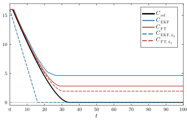
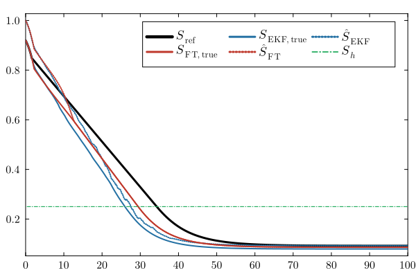
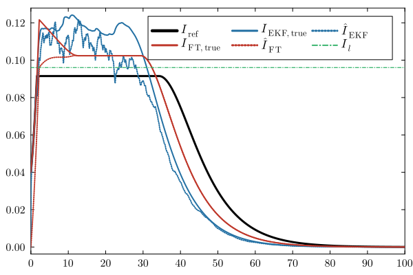
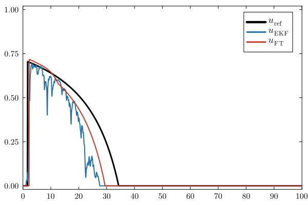
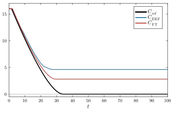
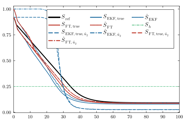
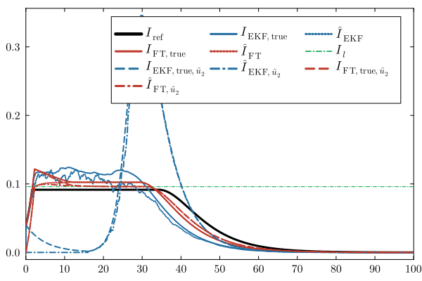
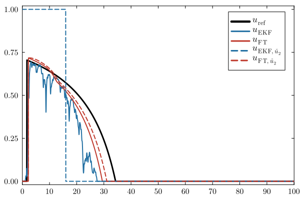
The following plots compare
- the susceptible population,
- the infected population,
- the feedback control,
- the remaining intervention budget.
The reference trajectory is shown together with the EKF-based and finite-time-observer-based closed-loop trajectories.
COLOR_REF =
    :black

COLOR_EKF =
    RGB(
        0.14,
        0.44,
        0.64
    )

COLOR_FT =
    RGB(
        0.75,
        0.22,
        0.17
    )

COLOR_SH =
    RGB(
        0.15,
        0.68,
        0.38
    )
nothing
Common plotting options are
common = (
    guidefontsize = 13,
    tickfontsize = 10,
    legendfontsize = 12,
    framestyle = :box,
    grid = false,
    xticks = 0:10:tf,
    xlims = (0, tf),
    left_margin = 0Plots.mm,
    right_margin = 1Plots.mm,
    dpi = 500
)
nothing
Susceptible population
pS =
    plot(
        t_ref,
        S_ref;

        lw = 3.0,
        color = COLOR_REF,

        label =
            L"S_{\mathrm{ref}}",

        legend = :topright,
        legend_column = 3,

        top_margin =
            3Plots.mm,

        bottom_margin =
            1Plots.mm,

        common...
    )

plot!(
    pS,
    t_ekf,
    S_ekf;

    lw = 2.0,
    color = COLOR_EKF,
    ls = :solid,

    label =
        L"S_{\mathrm{EKF,true}}"
)

plot!(
    pS,
    t_ekf,
    Shat_ekf;

    lw = 2.0,
    color = COLOR_EKF,
    ls = :dot,

    label =
        L"\hat S_{\mathrm{EKF}}"
)

plot!(
    pS,
    t_ft,
    S_ft;

    lw = 2.0,
    color = COLOR_FT,
    ls = :solid,

    label =
        L"S_{\mathrm{FT,true}}"
)

plot!(
    pS,
    t_ft,
    Shat_ft;

    lw = 2.0,
    color = COLOR_FT,
    ls = :dot,

    label =
        L"\hat S_{\mathrm{FT}}"
)

hline!(
    pS,
    [Sh];

    lw = 1.2,
    color = COLOR_SH,
    ls = :dashdot,

    label =
        L"S_h"
)
Infected population
pI =
    plot(
        t_ref,
        I_ref;

        lw = 3.0,
        color = COLOR_REF,

        label =
            L"I_{\mathrm{ref}}",

        legend = :topright,
        legend_column = 3,

        top_margin =
            1Plots.mm,

        bottom_margin =
            1Plots.mm,

        common...
    )

plot!(
    pI,
    t_ekf,
    I_ekf;

    lw = 2.0,
    color = COLOR_EKF,
    ls = :solid,

    label =
        L"I_{\mathrm{EKF,true}}"
)

plot!(
    pI,
    t_ekf,
    Ihat_ekf;

    lw = 2.0,
    color = COLOR_EKF,
    ls = :dot,

    label =
        L"\hat I_{\mathrm{EKF}}"
)

plot!(
    pI,
    t_ft,
    I_ft;

    lw = 2.0,
    color = COLOR_FT,
    ls = :solid,

    label =
        L"I_{\mathrm{FT,true}}"
)

plot!(
    pI,
    t_ft,
    Ihat_ft;

    lw = 2.0,
    color = COLOR_FT,
    ls = :dot,

    label =
        L"\hat I_{\mathrm{FT}}"
)

hline!(
    pI,
    [Il];

    lw = 1.2,
    color = COLOR_SH,
    ls = :dashdot,

    label =
        L"I_l"
)
Control
pU =
    plot(
        t_ref,
        u_ref;

        lw = 3.0,
        color = COLOR_REF,

        label =
            L"u_{\mathrm{ref}}",

        ylims =
            (-0.02, 1.02),

        legend =
            :topright,

        top_margin =
            1Plots.mm,

        bottom_margin =
            1Plots.mm,

        common...
    )

plot!(
    pU,
    t_ekf,
    u_ekf;

    lw = 2.0,
    color = COLOR_EKF,
    ls = :solid,

    label =
        L"u_{\mathrm{EKF}}"
)

plot!(
    pU,
    t_ft,
    u_ft;

    lw = 2.0,
    color = COLOR_FT,
    ls = :solid,

    label =
        L"u_{\mathrm{FT}}"
)
Remaining budget
pC =
    plot(
        t_ref,
        C_ref;

        lw = 3.0,
        color = COLOR_REF,

        label =
            L"C_{\mathrm{ref}}",

        xlabel =
            L"t",

        ylims =
            (-0.5, Qbudget + 1),

        legend =
            :topright,

        top_margin =
            1Plots.mm,

        bottom_margin =
            4Plots.mm,

        common...
    )

plot!(
    pC,
    t_ekf,
    C_ekf;

    lw = 2.0,
    color = COLOR_EKF,
    ls = :solid,

    label =
        L"C_{\mathrm{EKF}}"
)

plot!(
    pC,
    t_ft,
    C_ft;

    lw = 2.0,
    color = COLOR_FT,
    ls = :solid,

    label =
        L"C_{\mathrm{FT}}"
)

hline!(
    pC,
    [0.0];

    lw = 1.0,
    color = :gray,
    ls = :dot,

    label =
        false
)
Modified feedback trajectories
The closed-loop trajectories obtained with $\widetilde u_2$ are added to the same panels using dashed line styles.
plot!(
    pS,
    t_ekf_ut,
    S_ekf_ut;

    lw = 2.0,
    color = COLOR_EKF,
    ls = :dash,

    label =
        L"S_{\mathrm{EKF,true},\widetilde u_2}"
)

plot!(
    pS,
    t_ekf_ut,
    Shat_ekf_ut;

    lw = 2.0,
    color = COLOR_EKF,
    ls = :dashdot,

    label =
        L"\hat S_{\mathrm{EKF},\widetilde u_2}"
)

plot!(
    pS,
    t_ft_ut,
    S_ft_ut;

    lw = 2.0,
    color = COLOR_FT,
    ls = :dash,

    label =
        L"S_{\mathrm{FT,true},\widetilde u_2}"
)

plot!(
    pS,
    t_ft_ut,
    Shat_ft_ut;

    lw = 2.0,
    color = COLOR_FT,
    ls = :dashdot,

    label =
        L"\hat S_{\mathrm{FT},\widetilde u_2}"
)
plot!(
    pI,
    t_ekf_ut,
    I_ekf_ut;

    lw = 2.0,
    color = COLOR_EKF,
    ls = :dash,

    label =
        L"I_{\mathrm{EKF,true},\widetilde u_2}"
)

plot!(
    pI,
    t_ekf_ut,
    Ihat_ekf_ut;

    lw = 2.0,
    color = COLOR_EKF,
    ls = :dashdot,

    label =
        L"\hat I_{\mathrm{EKF},\widetilde u_2}"
)

plot!(
    pI,
    t_ft_ut,
    I_ft_ut;

    lw = 2.0,
    color = COLOR_FT,
    ls = :dash,

    label =
        L"I_{\mathrm{FT,true},\widetilde u_2}"
)

plot!(
    pI,
    t_ft_ut,
    Ihat_ft_ut;

    lw = 2.0,
    color = COLOR_FT,
    ls = :dashdot,

    label =
        L"\hat I_{\mathrm{FT},\widetilde u_2}"
)
plot!(
    pU,
    t_ekf_ut,
    u_ekf_ut;

    lw = 2.0,
    color = COLOR_EKF,
    ls = :dash,

    label =
        L"u_{\mathrm{EKF},\widetilde u_2}"
)

plot!(
    pU,
    t_ft_ut,
    u_ft_ut;

    lw = 2.0,
    color = COLOR_FT,
    ls = :dash,

    label =
        L"u_{\mathrm{FT},\widetilde u_2}"
)
plot!(
    pC,
    t_ekf_ut,
    C_ekf_ut;

    lw = 2.0,
    color = COLOR_EKF,
    ls = :dash,

    label =
        L"C_{\mathrm{EKF},\widetilde u_2}"
)

plot!(
    pC,
    t_ft_ut,
    C_ft_ut;

    lw = 2.0,
    color = COLOR_FT,
    ls = :dash,

    label =
        L"C_{\mathrm{FT},\widetilde u_2}"
)